Show the code
pacman::p_load(plotly, ggplot2, timetk, scales, viridis, lubridate, ggthemes, gridExtra, readxl, knitr, data.table, CGPfunctions, ggHoriPlot, tidyverse,funModeling)In this take-home exercise, we are required to uncover the impact of COVID-19 as well as the global economic and political dynamic in 2022 on Singapore bi-lateral trade (i.e. Import, Export and Trade Balance) by using appropriate analytical visualisation techniques learned in Lesson 6: It’s About Time. Students are encouraged to apply appropriate interactive techniques to enhance user and data discovery experiences.
For the purpose of this take-home exercise, Merchandise Trade provided by Department of Statistics, Singapore (DOS) will be used. The data are available under the sub-section of Merchandise Trade by Region/Market. We should download the data by clicking on the link Download all in Excel on the same webpage. The study period should be between January 2020 to December 2022.
For the purpose of this take-home exercise, ggplot2 and its extension should be used to design the analytical visualisation. tidyverse family of packages should be used to prepare the data.
Before we get started, it is important for us to install the necessary R packages into R and launch these R packages into R environment.
The R packages needed for this exercise are as follows:
pacman::p_load(plotly, ggplot2, timetk, scales, viridis, lubridate, ggthemes, gridExtra, readxl, knitr, data.table, CGPfunctions, ggHoriPlot, tidyverse,funModeling)Import <- read_excel("data/outputFile.xlsx", sheet = "T1", skip = 9)
Export <- read_excel("data/outputFile.xlsx", sheet = "T2", skip = 9)select data from 2020 Jan to 2022 Dec.
Import_1 <- Import %>%
  select(1,3:38)%>%
filter(row_number()<92 & row_number()>1)Export_1 <- Export %>%
select(1,3:38.)%>%
filter(row_number()<120 & row_number()>1)Check if any missing values
skimr::skim(Import_1)| Name | Import_1 |
| Number of rows | 90 |
| Number of columns | 37 |
| _______________________ | |
| Column type frequency: | |
| character | 1 |
| numeric | 36 |
| ________________________ | |
| Group variables | None |
Variable type: character
| skim_variable | n_missing | complete_rate | min | max | empty | n_unique | whitespace |
|---|---|---|---|---|---|---|---|
| Data Series | 0 | 1 | 22 | 52 | 0 | 90 | 0 |
Variable type: numeric
| skim_variable | n_missing | complete_rate | mean | sd | p0 | p25 | p50 | p75 | p100 | hist |
|---|---|---|---|---|---|---|---|---|---|---|
| 2022 Dec | 0 | 1 | 586243.8 | 1368046.9 | 0 | 6475.38 | 48296.50 | 307285.0 | 7403998 | ▇▁▁▁▁ |
| 2022 Nov | 0 | 1 | 571033.4 | 1301748.3 | 0 | 6575.65 | 47146.00 | 323984.0 | 6773005 | ▇▁▁▁▁ |
| 2022 Oct | 0 | 1 | 603702.2 | 1400359.3 | 0 | 7424.25 | 63806.50 | 360812.2 | 7810503 | ▇▁▁▁▁ |
| 2022 Sep | 0 | 1 | 667836.1 | 1489183.4 | 0 | 10033.75 | 57056.00 | 384880.0 | 7405741 | ▇▁▁▁▁ |
| 2022 Aug | 0 | 1 | 671755.9 | 1505473.5 | 0 | 9132.50 | 51208.50 | 455167.2 | 7548001 | ▇▁▁▁▁ |
| 2022 Jul | 0 | 1 | 686508.2 | 1515344.2 | 0 | 9656.75 | 58018.00 | 445801.0 | 7792074 | ▇▁▁▁▁ |
| 2022 Jun | 0 | 1 | 682164.9 | 1581835.2 | 0 | 8749.75 | 69630.00 | 408044.5 | 7717915 | ▇▁▁▁▁ |
| 2022 May | 0 | 1 | 639902.7 | 1478007.1 | 0 | 6531.58 | 56812.00 | 447629.0 | 7486002 | ▇▁▁▁▁ |
| 2022 Apr | 0 | 1 | 642572.5 | 1466588.8 | 0 | 9290.00 | 70217.50 | 444242.5 | 7481265 | ▇▁▁▁▁ |
| 2022 Mar | 0 | 1 | 680540.6 | 1609795.4 | 0 | 7703.25 | 64959.50 | 404368.2 | 8912350 | ▇▁▁▁▁ |
| 2022 Feb | 0 | 1 | 546062.8 | 1277520.9 | 0 | 6197.60 | 41282.00 | 355951.0 | 6929035 | ▇▁▁▁▁ |
| 2022 Jan | 0 | 1 | 590077.8 | 1357593.5 | 0 | 9586.50 | 52396.00 | 318862.2 | 7163479 | ▇▁▁▁▁ |
| 2021 Dec | 0 | 1 | 635704.1 | 1553241.9 | 0 | 10139.25 | 56858.00 | 320817.0 | 9215862 | ▇▁▁▁▁ |
| 2021 Nov | 0 | 1 | 608560.5 | 1474650.5 | 0 | 8109.50 | 55961.50 | 336858.2 | 8281345 | ▇▁▁▁▁ |
| 2021 Oct | 0 | 1 | 578280.1 | 1393269.2 | 0 | 7423.75 | 50327.50 | 372287.2 | 8461516 | ▇▁▁▁▁ |
| 2021 Sep | 0 | 1 | 561719.2 | 1422245.6 | 0 | 7359.50 | 48116.50 | 241825.8 | 8785105 | ▇▁▁▁▁ |
| 2021 Aug | 0 | 1 | 562337.3 | 1391492.2 | 0 | 7536.00 | 54621.50 | 251813.0 | 8134968 | ▇▁▁▁▁ |
| 2021 Jul | 0 | 1 | 536820.2 | 1305877.2 | 0 | 8512.75 | 40744.90 | 346546.8 | 7991895 | ▇▁▁▁▁ |
| 2021 Jun | 0 | 1 | 535805.9 | 1282636.4 | 0 | 7159.00 | 45186.00 | 356035.8 | 7300460 | ▇▁▁▁▁ |
| 2021 May | 0 | 1 | 510561.5 | 1277424.5 | 0 | 4913.75 | 41337.00 | 230461.0 | 7161940 | ▇▁▁▁▁ |
| 2021 Apr | 0 | 1 | 543848.6 | 1330817.3 | 0 | 6076.80 | 43846.00 | 287915.0 | 7838848 | ▇▁▁▁▁ |
| 2021 Mar | 0 | 1 | 595467.7 | 1412024.8 | 0 | 6628.00 | 41011.70 | 359609.2 | 7470910 | ▇▁▁▁▁ |
| 2021 Feb | 0 | 1 | 460230.5 | 1061792.0 | 0 | 5578.25 | 35105.50 | 284150.5 | 5518278 | ▇▁▁▁▁ |
| 2021 Jan | 0 | 1 | 487403.0 | 1122842.9 | 0 | 5970.75 | 42248.00 | 337218.8 | 5693673 | ▇▁▁▁▁ |
| 2020 Dec | 0 | 1 | 500637.4 | 1244183.6 | 0 | 6825.50 | 35537.90 | 219175.2 | 7090834 | ▇▁▁▁▁ |
| 2020 Nov | 0 | 1 | 468219.2 | 1169362.9 | 0 | 6485.75 | 36915.00 | 244342.5 | 6852887 | ▇▁▁▁▁ |
| 2020 Oct | 0 | 1 | 476473.3 | 1169379.8 | 0 | 5673.25 | 35167.45 | 255064.2 | 6992713 | ▇▁▁▁▁ |
| 2020 Sep | 0 | 1 | 473427.6 | 1141417.2 | 0 | 5206.77 | 34522.15 | 249263.5 | 6561515 | ▇▁▁▁▁ |
| 2020 Aug | 0 | 1 | 475320.8 | 1194167.0 | 0 | 5240.23 | 31650.25 | 243462.5 | 7970167 | ▇▁▁▁▁ |
| 2020 Jul | 0 | 1 | 464059.9 | 1141729.3 | 0 | 4713.25 | 32678.00 | 242386.5 | 5935191 | ▇▁▁▁▁ |
| 2020 Jun | 0 | 1 | 439898.8 | 1041629.8 | 0 | 4884.17 | 31531.00 | 215720.0 | 5603145 | ▇▁▁▁▁ |
| 2020 May | 0 | 1 | 394076.4 | 986818.5 | 0 | 4120.50 | 22439.40 | 180320.5 | 5080433 | ▇▁▁▁▁ |
| 2020 Apr | 0 | 1 | 429729.4 | 1068014.7 | 0 | 4385.75 | 26420.35 | 202348.5 | 5439082 | ▇▁▁▁▁ |
| 2020 Mar | 0 | 1 | 488955.1 | 1134882.1 | 0 | 5154.25 | 35816.00 | 330576.5 | 5823657 | ▇▁▁▁▁ |
| 2020 Feb | 0 | 1 | 462422.8 | 1002846.1 | 0 | 5214.97 | 42334.50 | 321633.8 | 5116584 | ▇▁▁▁▁ |
| 2020 Jan | 0 | 1 | 473619.4 | 1067404.8 | 0 | 5695.60 | 49916.50 | 268527.0 | 5091217 | ▇▁▁▁▁ |
skimr::skim(Export_1)| Name | Export_1 |
| Number of rows | 118 |
| Number of columns | 37 |
| _______________________ | |
| Column type frequency: | |
| character | 1 |
| numeric | 36 |
| ________________________ | |
| Group variables | None |
Variable type: character
| skim_variable | n_missing | complete_rate | min | max | empty | n_unique | whitespace |
|---|---|---|---|---|---|---|---|
| Data Series | 0 | 1 | 22 | 53 | 0 | 118 | 0 |
Variable type: numeric
| skim_variable | n_missing | complete_rate | mean | sd | p0 | p25 | p50 | p75 | p100 | hist |
|---|---|---|---|---|---|---|---|---|---|---|
| 2022 Dec | 0 | 1 | 418097.0 | 1194617.4 | 0 | 147.75 | 8210.50 | 118369.00 | 7642587 | ▇▁▁▁▁ |
| 2022 Nov | 0 | 1 | 423407.0 | 1272510.2 | 0 | 258.75 | 8015.70 | 120419.50 | 8285837 | ▇▁▁▁▁ |
| 2022 Oct | 0 | 1 | 444276.7 | 1284320.0 | 0 | 171.25 | 8924.00 | 145353.50 | 7377473 | ▇▁▁▁▁ |
| 2022 Sep | 0 | 1 | 467633.1 | 1334807.8 | 0 | 259.00 | 9367.50 | 143109.00 | 7672003 | ▇▁▁▁▁ |
| 2022 Aug | 0 | 1 | 489468.8 | 1414702.8 | 0 | 203.25 | 9749.00 | 160920.00 | 8196629 | ▇▁▁▁▁ |
| 2022 Jul | 0 | 1 | 510922.4 | 1446098.1 | 0 | 427.75 | 8572.25 | 180595.00 | 8510236 | ▇▁▁▁▁ |
| 2022 Jun | 0 | 1 | 498639.8 | 1431575.1 | 0 | 246.50 | 11288.50 | 165379.00 | 7976196 | ▇▁▁▁▁ |
| 2022 May | 0 | 1 | 484051.5 | 1367418.0 | 0 | 160.00 | 8995.00 | 158037.25 | 7478079 | ▇▁▁▁▁ |
| 2022 Apr | 0 | 1 | 468073.3 | 1303380.5 | 0 | 128.75 | 8904.00 | 139441.00 | 6958619 | ▇▁▁▁▁ |
| 2022 Mar | 0 | 1 | 485301.3 | 1388471.4 | 0 | 140.25 | 7754.00 | 143188.00 | 7882249 | ▇▁▁▁▁ |
| 2022 Feb | 0 | 1 | 373312.6 | 1046659.0 | 0 | 100.25 | 6967.50 | 157869.00 | 6469836 | ▇▁▁▁▁ |
| 2022 Jan | 0 | 1 | 417040.6 | 1182252.6 | 0 | 106.75 | 9321.50 | 136106.75 | 6978727 | ▇▁▁▁▁ |
| 2021 Dec | 0 | 1 | 454829.1 | 1310774.4 | 0 | 193.25 | 8350.50 | 121241.00 | 7876015 | ▇▁▁▁▁ |
| 2021 Nov | 0 | 1 | 420205.3 | 1196997.8 | 0 | 161.75 | 7770.50 | 132750.00 | 6670871 | ▇▁▁▁▁ |
| 2021 Oct | 0 | 1 | 398616.9 | 1134627.2 | 0 | 162.75 | 6626.90 | 153802.75 | 6447589 | ▇▁▁▁▁ |
| 2021 Sep | 0 | 1 | 384251.1 | 1112802.3 | 0 | 104.75 | 7500.50 | 160929.50 | 6184737 | ▇▁▁▁▁ |
| 2021 Aug | 0 | 1 | 370593.3 | 1084077.8 | 0 | 87.50 | 7024.50 | 125688.25 | 6519894 | ▇▁▁▁▁ |
| 2021 Jul | 0 | 1 | 384216.1 | 1072829.6 | 0 | 170.00 | 7928.00 | 136928.75 | 6094544 | ▇▁▁▁▁ |
| 2021 Jun | 0 | 1 | 372826.9 | 1046044.3 | 0 | 55.75 | 6234.30 | 143808.75 | 6198485 | ▇▁▁▁▁ |
| 2021 May | 0 | 1 | 347202.6 | 1004935.6 | 0 | 134.50 | 6421.25 | 139041.75 | 5932710 | ▇▁▁▁▁ |
| 2021 Apr | 0 | 1 | 375263.6 | 1095326.9 | 0 | 125.75 | 7301.75 | 125678.50 | 6329544 | ▇▁▁▁▁ |
| 2021 Mar | 0 | 1 | 393168.7 | 1094654.3 | 0 | 119.50 | 8530.50 | 126112.75 | 6291717 | ▇▁▁▁▁ |
| 2021 Feb | 0 | 1 | 310132.2 | 900528.0 | 0 | 74.50 | 5349.50 | 86724.00 | 5402465 | ▇▁▁▁▁ |
| 2021 Jan | 0 | 1 | 325242.2 | 976314.0 | 0 | 87.00 | 7120.50 | 115283.00 | 6121009 | ▇▁▁▁▁ |
| 2020 Dec | 0 | 1 | 333250.8 | 974409.3 | 0 | 169.75 | 7174.00 | 130818.50 | 6202327 | ▇▁▁▁▁ |
| 2020 Nov | 0 | 1 | 319340.5 | 938043.2 | 0 | 116.75 | 5735.25 | 133326.25 | 6280686 | ▇▁▁▁▁ |
| 2020 Oct | 0 | 1 | 317425.3 | 925927.0 | 0 | 80.50 | 5345.50 | 124435.75 | 5249328 | ▇▁▁▁▁ |
| 2020 Sep | 0 | 1 | 324791.5 | 925020.3 | 0 | 122.50 | 7756.00 | 93170.50 | 5479579 | ▇▁▁▁▁ |
| 2020 Aug | 0 | 1 | 303788.9 | 885364.5 | 0 | 144.25 | 6057.50 | 95664.00 | 5574117 | ▇▁▁▁▁ |
| 2020 Jul | 0 | 1 | 316079.8 | 906421.6 | 0 | 171.00 | 8152.50 | 113675.25 | 5539168 | ▇▁▁▁▁ |
| 2020 Jun | 0 | 1 | 293978.1 | 887991.3 | 0 | 112.00 | 4823.45 | 93924.50 | 5288235 | ▇▁▁▁▁ |
| 2020 May | 0 | 1 | 262592.9 | 773859.1 | 0 | 39.50 | 4444.00 | 95021.25 | 4843684 | ▇▁▁▁▁ |
| 2020 Apr | 0 | 1 | 299137.5 | 864578.2 | 0 | 31.00 | 5167.05 | 95948.75 | 5583246 | ▇▁▁▁▁ |
| 2020 Mar | 0 | 1 | 336379.9 | 950555.8 | 0 | 112.25 | 6413.15 | 116936.25 | 5979894 | ▇▁▁▁▁ |
| 2020 Feb | 0 | 1 | 325768.8 | 860980.8 | 0 | 132.75 | 7261.50 | 147114.25 | 4985932 | ▇▁▁▁▁ |
| 2020 Jan | 0 | 1 | 339509.0 | 914691.7 | 0 | 100.25 | 6510.35 | 122115.50 | 5469816 | ▇▁▁▁▁ |
Separate the country and thousand/million
Import_2 <- Import_1 %>%
  separate(`Data Series`, c("country", "unit"),
           sep = ' \\(T|\\(M') %>%
mutate(unit = str_remove(unit, '\\)'))Export_2 <- Export_1 %>%
separate(`Data Series`, c("country", "unit"),
sep = ' \\(T|\\(M') %>%
mutate(unit = str_remove(unit, '\\)'))ImportK is Import data by thousand/countries.
ImportK <- Import_2 %>%
  filter(str_detect(unit, "housand")) %>%
  select(-(unit))
ImportM is Import data by million/regions.
ImportM <- Import_2 %>%
  filter(str_detect(unit, "illion")) %>%
  select(-(unit))
ExportK is Export data by thousand/countries.
ExportK<- Export_2 %>%
  filter(str_detect(unit, "housand")) %>%
  select(-(unit))
ExportM is Export data by million/regions.
ExportM<- Export_2 %>%
  filter(str_detect(unit, "illion")) %>%
  select(-(unit))
Create pivot table to list down the date period in the same column.
ImportK_pvL <- ImportK %>%
  pivot_longer(cols = !country,
               names_to = "temporary",
               values_to = "import") %>%
  mutate(period = (lubridate::ym(temporary))) %>%
  arrange(country, period)

ImportK_pvL <- ImportK_pvL %>%
  mutate(month = factor(month
                        (ImportK_pvL$`period`),
                        levels = 1:12,
                        labels = month.abb,
                        ordered = TRUE)) %>%
  mutate(year = as.character(year(ymd(ImportK_pvL$`period`)))) %>%
  relocate(year, month) %>%
  select(-temporary)%>%
  arrange(desc(import))
Create pivot table to list down the date period in the same column.
ImportM_pvL <- ImportM %>%
  pivot_longer(cols = !country,
               names_to = "temporary",
               values_to = "import") %>%
  mutate(period = (lubridate::ym(temporary))) %>%
  arrange(country, period)

ImportM_pvL <- ImportM_pvL %>%
  mutate(month = factor(month
                        (ImportM_pvL$`period`),
                        levels = 1:12,
                        labels = month.abb,
                        ordered = TRUE)) %>%
  mutate(year = as.character(year(ymd(ImportM_pvL$`period`)))) %>%
  relocate(year, month) %>%
  select(-temporary)%>%
  arrange(desc(import))
Create pivot table to list down the date period in the same column.
ExportK_pvL <- ExportK %>%
  pivot_longer(cols = !country,
               names_to = "temporary",
               values_to = "export") %>%
  mutate(period = (lubridate::ym(temporary))) %>%
  arrange(country, period)

ExportK_pvL<- ExportK_pvL %>%
  mutate(month = factor(month
                        (ExportK_pvL$`period`),
                        levels = 1:12,
                        labels = month.abb,
                        ordered = TRUE)) %>%
  mutate(year = as.character(year(ymd(ExportK_pvL$`period`)))) %>%
  relocate(year, month) %>%
  select(-temporary)%>%
  arrange(desc(export))
Create pivot table to list down the date period in the same column.
ExportM_pvL <- ExportM %>%
  pivot_longer(cols = !country,
               names_to = "temporary",
               values_to = "export") %>%
  mutate(period = (lubridate::ym(temporary))) %>%
  arrange(country, period)

ExportM_pvL<- ExportM_pvL %>%
  mutate(month = factor(month
                        (ExportM_pvL$`period`),
                        levels = 1:12,
                        labels = month.abb,
                        ordered = TRUE)) %>%
  mutate(year = as.character(year(ymd(ExportM_pvL$`period`)))) %>%
  relocate(year, month) %>%
  select(-temporary)%>%
  arrange(desc(export))
Merge import and export by countries.
TradeK<- ImportK_pvL %>%
  full_join(ExportK_pvL)%>%
  mutate(trade_total = import + export)%>%
  mutate(formatted_period = format(period, "%Y %B"))%>%
  mutate(trade_balance = export - import)
Merge import and export by regions.
TradeM<- ImportM_pvL %>%
  full_join(ExportM_pvL)%>%
  mutate(trade_total = import + export)%>%
  mutate(formatted_period = format(period, "%Y %B"))%>%
  mutate(trade_balance = export - import)
By countries: List “import” and “export” in the same column, name as “Type”, select the column that we need for further analysis, and filter the total trade >10000 million per country.
Trade_country<- TradeK %>%
  pivot_longer(cols = c("import","export"),
               names_to = "Type",
               values_to = "Amount") %>%
  na.omit("Amount")%>%
  group_by(country)%>%
  summarise(year,
            month,
            country,
            trade_country = sum(trade_total/1000),
            period,
            formatted_period,
            Type,

            Amount = round(Amount/1000)) %>%
  arrange(desc(trade_country))%>%
  filter(trade_country > 10000)
By regions: List “import” and “export” in the same column, name as “Type”, select the column that we need for further analysis
Trade_region<- TradeM %>%
  pivot_longer(cols = c("import","export"),
               names_to = "Type",
               values_to = "Amount") %>%
  na.omit("Amount")%>%
  group_by(country)%>%
  summarise(year,
            month,
            country,
            trade_country = sum(trade_total),
            period,
            formatted_period,
            Type,
            Amount) %>%
  arrange(desc(trade_country))
Examine the final data set.
summary(Trade_country) country year month trade_country
Length:2736 Length:2736 Jan : 228 Min. : 11194
Class :character Class :character Feb : 228 1st Qu.: 28868
Mode :character Mode :character Mar : 228 Median : 78635
Apr : 228 Mean :174271
May : 228 3rd Qu.:161824
Jun : 228 Max. :950965
(Other):1368
period formatted_period Type Amount
Min. :2020-01-01 Length:2736 Length:2736 Min. : 0
1st Qu.:2020-09-23 Class :character Class :character 1st Qu.: 128
Median :2021-06-16 Mode :character Mode :character Median : 457
Mean :2021-06-16 Mean :1210
3rd Qu.:2022-03-08 3rd Qu.:1445
Max. :2022-12-01 Max. :9216
glimpse(Trade_country)Rows: 2,736
Columns: 8
Groups: country [38]
$ country <chr> "Mainland China", "Mainland China", "Mainland China",…
$ year <chr> "2021", "2021", "2022", "2022", "2021", "2021", "2021…
$ month <ord> Dec, Dec, Mar, Mar, Sep, Sep, Oct, Oct, Nov, Nov, Aug…
$ trade_country <dbl> 950965.3, 950965.3, 950965.3, 950965.3, 950965.3, 950…
$ period <date> 2021-12-01, 2021-12-01, 2022-03-01, 2022-03-01, 2021…
$ formatted_period <chr> "2021 December", "2021 December", "2022 March", "2022…
$ Type <chr> "import", "export", "import", "export", "import", "ex…
$ Amount <dbl> 9216, 7876, 8912, 6636, 8785, 6017, 8462, 6026, 8281,…summary(Trade_region) country year month trade_country
Length:432 Length:432 Jan : 36 Min. : 95298
Class :character Class :character Feb : 36 1st Qu.: 241065
Mode :character Mode :character Mar : 36 Median : 723092
Apr : 36 Mean :1266720
May : 36 3rd Qu.: 862475
Jun : 36 Max. :4955298
(Other):216
period formatted_period Type Amount
Min. :2020-01-01 Length:432 Length:432 Min. : 238.2
1st Qu.:2020-09-23 Class :character Class :character 1st Qu.: 1540.2
Median :2021-06-16 Mode :character Mode :character Median : 4680.8
Mean :2021-06-16 Mean : 8796.7
3rd Qu.:2022-03-08 3rd Qu.: 6718.9
Max. :2022-12-01 Max. :46328.8
glimpse(Trade_region)Rows: 432
Columns: 8
Groups: country [6]
$ country <chr> "Asia ", "Asia ", "Asia ", "Asia ", "Asia ", "Asia ",…
$ year <chr> "2022", "2022", "2022", "2022", "2022", "2022", "2022…
$ month <ord> Jun, Jun, Jul, Jul, Sep, Sep, Mar, Mar, Dec, Dec, Aug…
$ trade_country <dbl> 4955298, 4955298, 4955298, 4955298, 4955298, 4955298,…
$ period <date> 2022-06-01, 2022-06-01, 2022-07-01, 2022-07-01, 2022…
$ formatted_period <chr> "2022 June", "2022 June", "2022 July", "2022 July", "…
$ Type <chr> "import", "export", "import", "export", "import", "ex…
$ Amount <dbl> 46328.8, 42507.2, 46129.5, 43214.2, 45605.1, 37696.3,…cp_region <- ggplot(data = Trade_region, aes(x = period, y = Amount)) +
geom_line(aes(colour = Type)) +
labs(x = "Date", y = "Amount", title = "Imports & Exports by Region, 2022") +
facet_wrap(~ country) +
theme_bw() +
theme(plot.title = element_text(hjust = 0.5))
ggplotly(cp_region)From the above chart, we can see that Asia shows most significant import and export trade relation with Singapore since year 2020 to 2022, followed by Europe, European union, Oceania. Asia shows increasing trend during the mentioned time frame whereas Europe, European union, Oceania show stable trade trend. Hence, we will focus on about 80% of top trade with Singapore which are Asia and Europe.
cp_country <- ggplot(data = Trade_country, aes(x = period, y = Amount)) +
  geom_line(aes(colour = Type )) +
  labs(x = "Month", y = "Amount", title = "Imports & Exports by Region,  2022") +
  facet_wrap(~ country) +
  theme_bw() +
  theme(plot.title = element_text(hjust = 0.5))

ggplotly(cp_country)
From the above chart, we can observe that, Hong Kong, Indonesia, Mainland China, Malaysia, Republic of Korean,Switzerland,Taiwan, Thailand, United Arab Emirates,United Kingdom, United States, Vietnam, Socialist Republic are the top 10 countries which has most significant trade relation with Singapore from 2020 to 2022. We will further analyze these countries.
Trade_top10<- Trade_country %>%
filter(country %in% c("Mainland China", "Malaysia", "Republic of Korean", "Switzerland","Taiwan", "Thailand","United Arab Emirates","United Kingdom", "United States", "Vietnam, Socialist Republic Of" ))cp_top10 <- ggplot(data = Trade_top10, aes(x = period, y = Amount)) +
geom_line(aes(colour = Type)) +
labs(x = "Month", y = "Amount", title = "Imports & Exports by Region, 2022") +
facet_wrap(~ country) +
theme_bw() +
theme(plot.title = element_text(hjust = 0.5))
ggplotly(cp_top10)The above chart shows top 10 countries which have the most significant trade relation with Singapore. Mainland China, Malaysia, and Taiwan are the top 3 countries which showed increasing import and export trade.Whereas the Thailand, United Arab Emirates, United Kingdom, United States, Vietnam showed stable import and export trend.
ts_region <- TradeM%>%
  group_by(country) %>%
  plot_time_series(period, trade_balance,.color_var = year,  .facet_ncol = 2, .facet_scales = "free", .interactive = TRUE)
ggplotly(ts_region)
The following is the time series plot for trade balance(import-export) by region.
ts_top10 <- TradeK%>%
  group_by(country) %>%
  filter(country %in% c("Mainland China", "Malaysia", "Republic of Korean", "Switzerland","Taiwan", "Thailand","United Arab Emirates","United Kingdom", "United States", "Vietnam, Socialist Republic Of" ))%>%
  plot_time_series(period, trade_balance,.color_var = year,  .facet_ncol = 2, .facet_scales = "free", .interactive = TRUE)
ggplotly(ts_top10)
The following is the time series plot for trade balance(import-export) by top10 countries.
Trade_region %>%
  filter(Type == "import")%>%
  group_by(country, year) %>%
  summarise(Amount = sum(Amount)) %>%
  mutate(year = factor(year)) %>%
  filter(year %in% c(2020, 2021,2022)) %>%
  newggslopegraph(year, Amount, country,
                  Title = "Imports by Region",
                  SubTitle = "2020 to 2022",
                  Caption = "Source: Department of Statistics, Singapore")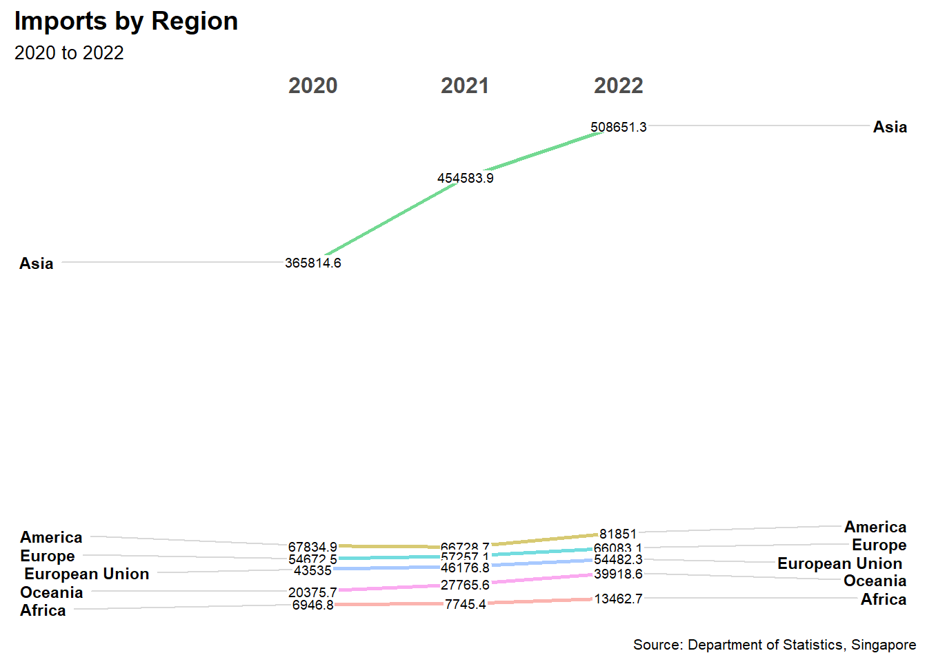
The above chart shows Asia has increasing trend of imports from year 2020 to 2022.
Trade_region %>%
  filter(Type == "export")%>%
  group_by(country, year) %>%
  summarise(Amount = sum(Amount)) %>%
  mutate(year = factor(year)) %>%
  filter(year %in% c(2020, 2021,2022)) %>%
  newggslopegraph(year, Amount, country,
                  Title = "Exports by Region",
                  SubTitle = "2020 to 2022",
                  Caption = "Source: Department of Statistics, Singapore")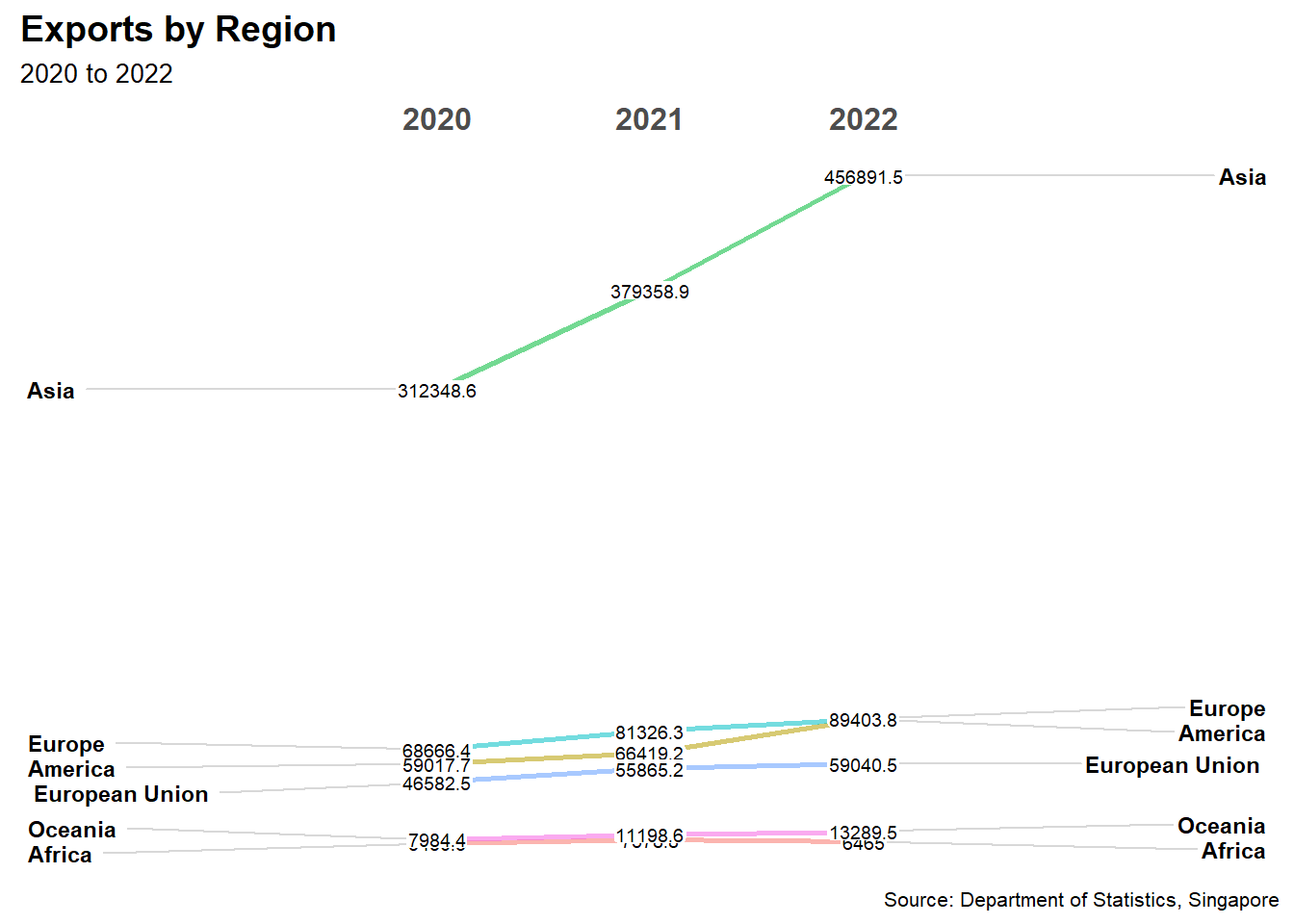
The above chart shows Asia has increasing trend of exports from year 2020 to 2022.
Trade_top10 %>%
  filter(Type == "import")%>%
  group_by(country, year) %>%
  summarise(Amount = sum(Amount)) %>%
  mutate(year = factor(year)) %>%
  filter(year %in% c(2020, 2021,2022)) %>%
  newggslopegraph(year, Amount, country,
                  Title = "Imports by top10 countries",
                  SubTitle = "2020 to 2022",
                  Caption = "Source: Department of Statistics, Singapore")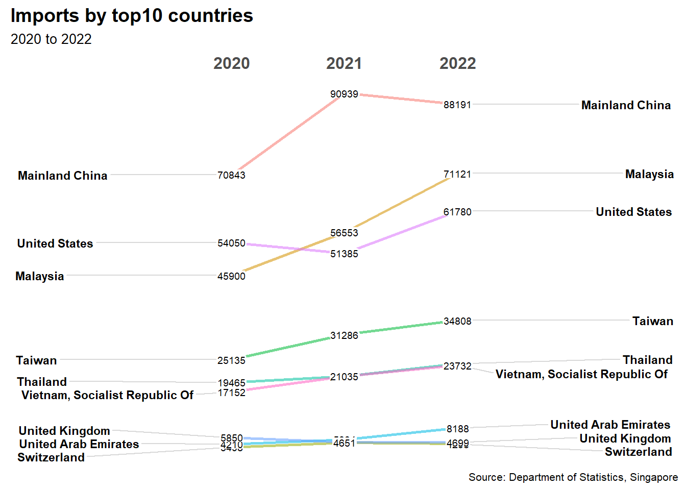
The above chart shows the imports trend of top10 countries which have most trade relation with Singapore.
Trade_top10 %>%
  filter(Type == "export")%>%
  group_by(country, year) %>%
  summarise(Amount = sum(Amount)) %>%
  mutate(year = factor(year)) %>%
  filter(year %in% c(2020, 2021,2022)) %>%
  newggslopegraph(year, Amount, country,
                  Title = "Exports by top10 countries",
                  SubTitle = "2020 to 2022",
                  Caption = "Source: Department of Statistics, Singapore")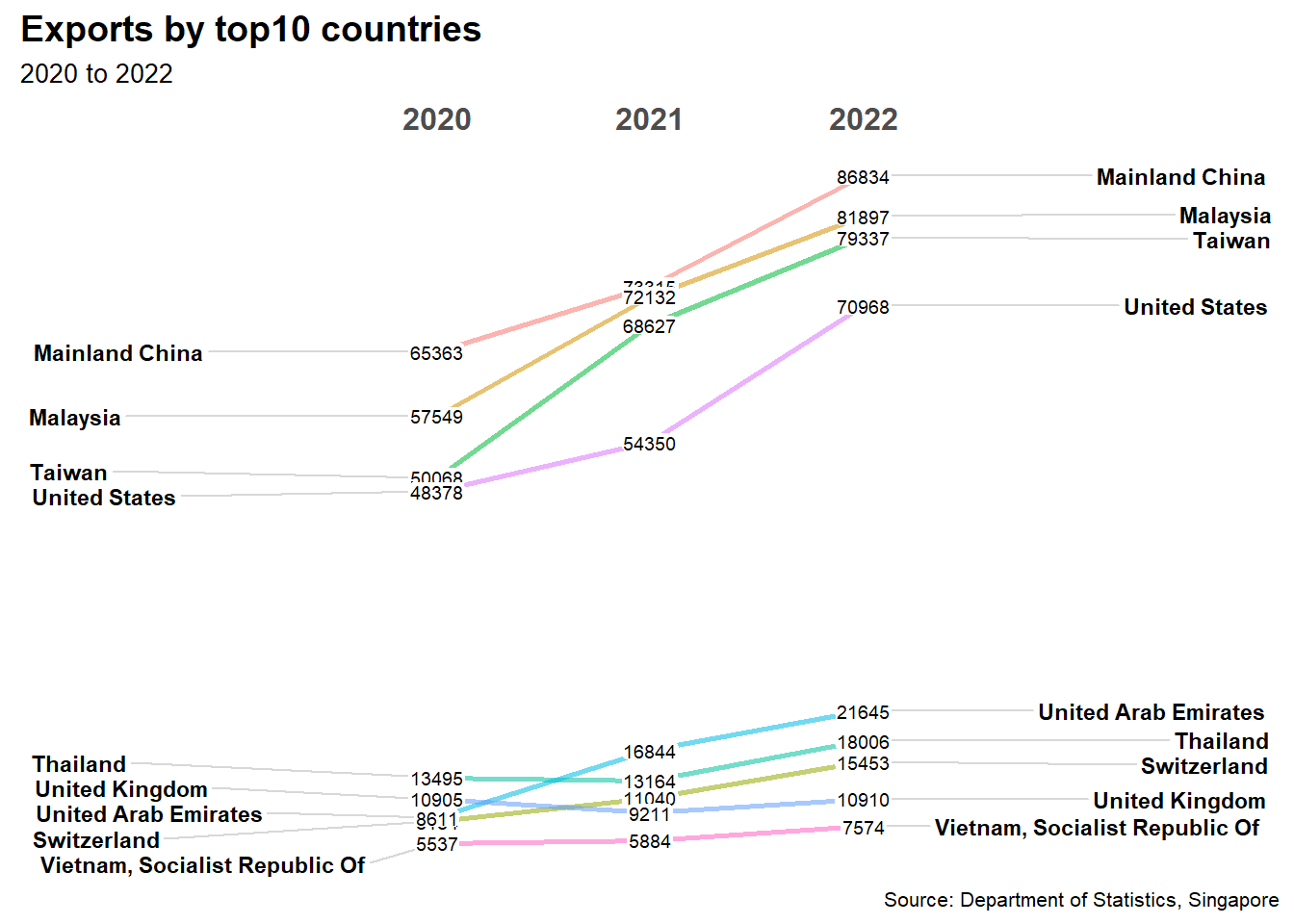
The above chart shows the exports trend of top10 countries which have most trade relation with Singapore.
TradeM %>%

  filter(period >= "2020-01-01") %>%
  ggplot() +
  geom_horizon(aes(x = period, y=trade_balance),
               origin = "midpoint",
               horizonscale = 6)+
  facet_grid(`country`~.) +
    theme_few() +
  scale_fill_hcl(palette = 'RdBu') +
  theme(panel.spacing.y=unit(0, "lines"), strip.text.y = element_text(
    size = 5, angle = 0, hjust = 0),
    legend.position = 'none',
    axis.text.y = element_blank(),
    axis.text.x = element_text(size=7),
    axis.title.y = element_blank(),
    axis.title.x = element_blank(),
    axis.ticks.y = element_blank(),
    panel.border = element_blank()
    ) +
    scale_x_date(expand=c(0,0), date_breaks = "3 month", date_labels = "%b%y") +
  ggtitle('Trade blance by region (Jan 2020 to Dec 2022)')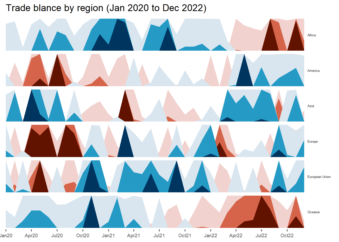
The chart shows there is large trade balance in Asia. The darker area, the larger balance.
TradeK %>%
  filter(country %in% c("Mainland China", "Malaysia", "Republic of Korean", "Switzerland","Taiwan", "Thailand","United Arab Emirates","United Kingdom", "United States", "Vietnam, Socialist Republic Of" ))%>%
  filter(period >= "2020-01-01") %>%
  ggplot() +
  geom_horizon(aes(x = period, y=trade_balance),
               origin = "midpoint",
               horizonscale = 6)+
  facet_grid(`country`~.) +
    theme_few() +
  scale_fill_hcl(palette = 'RdBu') +
  theme(panel.spacing.y=unit(0, "lines"), strip.text.y = element_text(
    size = 5, angle = 0, hjust = 0),
    legend.position = 'none',
    axis.text.y = element_blank(),
    axis.text.x = element_text(size=7),
    axis.title.y = element_blank(),
    axis.title.x = element_blank(),
    axis.ticks.y = element_blank(),
    panel.border = element_blank()
    ) +
    scale_x_date(expand=c(0,0), date_breaks = "3 month", date_labels = "%b%y") +
  ggtitle('Top 10 countries Trade blance (Jan 2020 to Dec 2022)')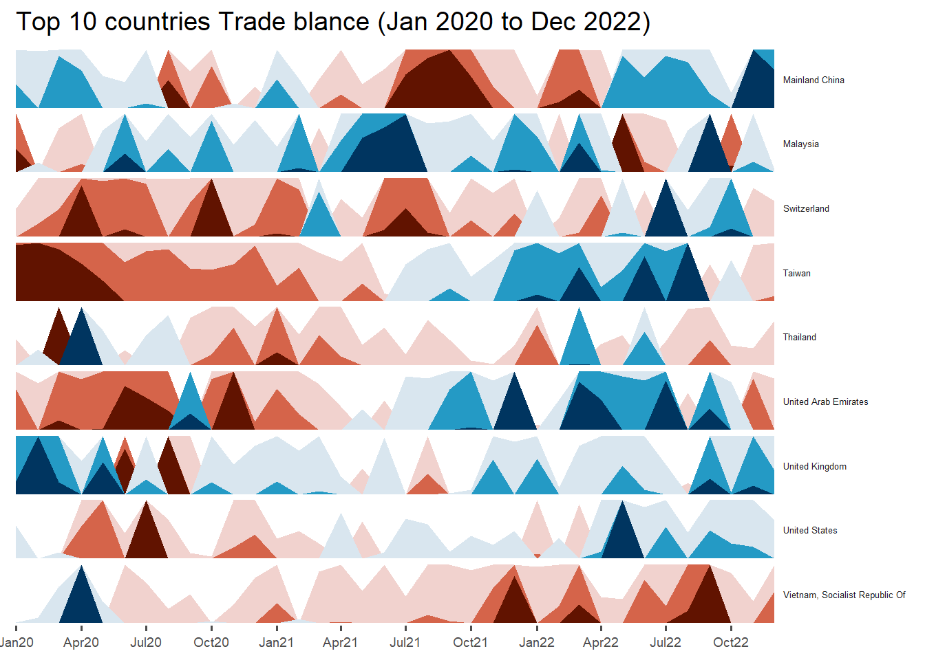
The chart shows there is large trade balance in Mainland China, Malaysia and Taiwan. The darker area, the larger balance.